Man, Economy, and State with Power and Market

What is the relationship between the APP and MPP? The MPP is the amount of physical product that will be produced with the addition of one unit of a factor, other factors being given. The APP is the ratio of the total product to the total quantity of the variable factor, other factors being given. To illustrate the meanings of APP and MPP, let us consider a hypothetical case in which all units of other factors are constant, and the number of units of one factor is variable. In Table 13 the first column lists the number of units of the variable factor, and the second column the total physical product produced when these varying units are combined with fixed units of the other factors. The third column is the APP = total product divided by the number of units of the factor, i.e., the average physical productivity of a unit of the factor. The fourth column is the MPP = the difference in total product yielded by adding one more unit of the variable factor, i.e., the total product of the current row minus the total product of the preceding row:

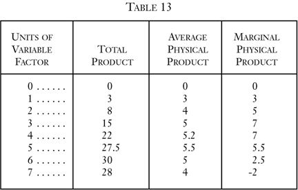
In the first place, it is quite clear that no factor will ever be employed in the region where the MPP is negative. In our example, this occurs where seven units of the factor are being employed. Six units of the factor, combined with given other factors, produced 30 units of the product. An addition of another unit results in a loss of two units of the product. The MPP of the factor when seven units are employed is -2. Obviously, no factor will ever be employed in this region, and this holds true whether the factor-owner is also owner of the product, or a capitalist hires the factor to work on the product. It would be senseless and contrary to the principles of human action to expend either effort or money on added factors only to have the quantity of the total product decline.

In the tabulation, we follow the law of returns, in that the APP, beginning, of course, at zero with zero units of the factor, rises to a peak and then falls. We also observe the following from our chart: (1) when the APP is rising (with the exception of the very first step where T P, APP, and MPP are all equal) MPP is higher than APP; (2) when the APP is falling, MPP is lower than APP; (3) at the point of maximum APP, MPP is equal to APP. We shall now prove, algebraically, that these three laws always hold.7

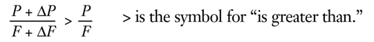
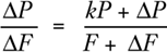
Let F be any number of units of a variable factor, other factors being given, and P be the units of the total product yielded by the combination. Then P/F is the Average Physical Product. When we add ΔF more units of the factor, total product increases by ΔP. Marginal Physical Product corresponding to the increase in the factor is ΔP/ΔF. The new Average Physical Product, corresponding to the greater supply of factors, is:

Now the new APP might be higher or lower than the previous one. Let us suppose that the new APP is higher and that therefore we are in a region where the APP is increasing. This means that:

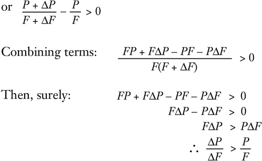
Thus, the MPP is greater than the old APP. Since it is greater, this means that there exists a positive number k such that:

Now there is an algebraic rule according to which, if:

then

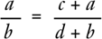
Therefore,

Since k is positive,

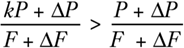
Therefore,

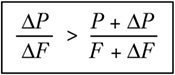
In short, the MPP is also greater than the new APP.

In other words, if APP is increasing, then the marginal physical product is greater than the average physical product in this region. This proves the first law above. Now, if we go back in our proof and substitute “less than” signs for “greater than” signs and carry out similar steps, we arrive at the opposite conclusion: where APP is decreasing, the marginal physical product is lower than the average physical product. This proves the second of our three laws about the relation between the marginal and the average physical product. But if MPP is greater than APP when the latter is rising, and is lower than APP when the latter is falling, then it follows that when APP is at its maximum, MPP must be neither lower nor higher than, but equal to, APP. And this proves the third law. We see that these characteristics of our table apply to all possible cases of production.

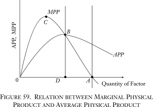
The diagram in Figure 59 depicts a typical set of MPP and APP schedules. It shows the various relationships between APP and MPP. Both curves begin from zero and are identical very close to their origin. The APP curve rises until it reaches a peak at B, then declines. The MPP curve rises faster, so that it is higher than APP, reaches its peak earlier at C, then declines until it intersects with APP at B. From then on, the MPP curve declines faster than APP, until finally it crosses the horizontal axis and becomes negative at some point A. No firm will operate beyond the 0A area.

Now let us explore further the area of increasing APP, between 0 and D. Let us take another hypothetical tabulation (Table 14), which will be simpler for our purpose.

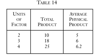
This is a segment of the increasing section of the average physical product schedule, with the peak being reached at four units and 6.2 APP. The question is: What is the likelihood that this region will be settled upon by a firm as the right input-output combination? Let us take the top line of the chart. Two units of the variable factor, plus a bundle of what we may call U units of all the other factors, yield 10 units of the product. On the other hand, at the maximum APP for the factor, four units of it, plus U units of other factors, yield 25 units of the product. We have seen above that it is a fundamental truth in nature that the same quantitative causes produce the same quantitative effects. Therefore, if we halve the quantities of all of the factors in the third line, we shall get half the product. In other words, two units of the factor combined with U/2—with half of the various units of each of the other factors—will yield 12.5 units of the product.

Consider this situation. From the top line we see that two units of the variable factor, plus U units of given factors, yield 10 units of the product. But, extrapolating from the bottom line, we see that two units of the variable factor, plus U/2 units of given factors, yield 12.5 units of the product. It is obvious that, as in the case of going beyond 0A, any firm that allocated factors so as to be in the 0D region would be making a most unwise decision. Obviously, no one would want to spend more in effort or money on factors (the “other” factors) and obtain less total output or, for that matter, the same total output. It is evident that if the producer remains in the 0D region, he is in an area of negative marginal physical productivity of the other factors. He would be in a situation where he would obtain a greater total product by throwing away some of the other factors. In the same way, after 0A, he would be in a position to gain greater total output if he threw away some of the present variable factor. A region of increasing APP for one factor, then, signifies a region of negative MPP for other factors, and vice versa. A producer, then, will never wish to allocate his factor in the 0D region or in the region beyond A.

Neither will the producer set the factor so that its MPP is at the points B or A. Indeed, the variable factor will be set so that it has zero marginal productivity (at A) only if it is a free good. There is however, no such thing as a free good; there is only a condition of human welfare not subject to action, and therefore not an element in productivity schedules. Conversely, the APP is at B, its maximum for the variable factor, only when the other factors are free goods and therefore have zero marginal productivity at this point. Only if all the other factors were free and could be left out of account could the producer simply concentrate on maximizing the productivity of one factor alone. However, there can be no production with only one factor, as we saw in chapter 1.

The conclusion, therefore, is inescapable. A factor will always be employed in a production process in such a way that it is in a region of declining APP and declining but positive MPP— between points D and A on the chart. In every production process, therefore, every factor will be employed in a region of diminishing MPP and diminishing APP so that additional units of the factor employed in the process will lower the MPP, and decreased units will raise it.

• 7It might be asked why we now employ mathematics after our strictures against the mathematical method in economics. The reason is that, in this particular problem, we are dealing with a purely technological question. We are not dealing with human decisions here, but with the necessary technological conditions of the world as given to human factors. In this external world, given quantities of cause yield given quantities of effect, and it is this sphere, very limited in the overall praxeological picture, that, like the natural sciences in general, is peculiarly susceptible to mathematical methods. The relationship between average and marginal is an obviously algebraic, rather than an ends-means, relation. Cf. the algebraic proof in Stigler, Theory of Price, pp. 44 ff.